Chapter 6 Tracking
At the end of the last chapter, I said, to measure the performance of an LP
position or a sequence of positions, I only use position PnL (pPnL) and
position APR (pAPR), which are defined as
pPnL= Current Liquidity Value - Initial Liquidity Value + Fees Earned - Gas.pAPR= Position PnL / Initial Liquidity Value / Position Age (days) * 365.
This chapter shows you how to do that in google sheets. Let’s get started.

Right after opening an LP position, we can calculate its Fee APR and track it continuously until we close the position. The following screen organizes Fee APR formulas chronologically.
Let’s see an example of Fee APR calculation at position close. First, we need to track a few items:
- position open time and close time,
- token prices at open time and close time,
- number of tokens sent to the pool at open time,
- number of tokens withdrawn from the pool at close time, and
- fees earned in each token.
We can then calculate
- duration in days,
- liquidity value at open time and close time,
- fees value at close time, and finally
- Fee APR at close time.
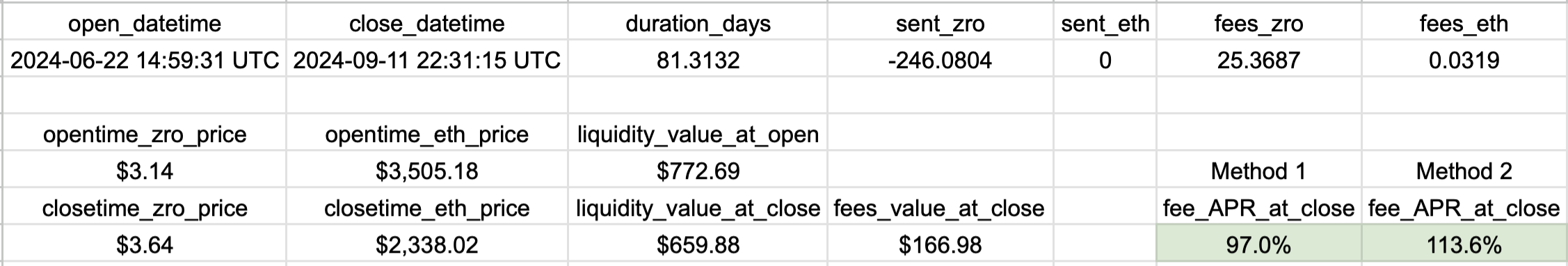
Notice method 1 and 2 give different results. Because we primarily use Fee APR to compare positions or pools, we care about their relative values way more than their absolute values. So we don’t need to make a fuss about which method to use, as long as we use the same method consistently. However, I do prefer to use method 1 because of common sense. But method 2 is more convenient since it doesn’t require open time prices. That’s why many DeFi applications use method 2 for real time Fee APR calculations.
In practice, we rarely need to calculate Fee APR of any single position since most DEXes display it automatically, or in the case of Uniswap V3 positions, we can track them at revert finance (https://revert.finance). But we do need to calculate it ourselves if we want to know the overall Fee APR across multiple positions. For example, the screen below shows 11 USDC-SOL positions between December 7 and 24 in 2023. I started this train of positions with $2500. The last two columns record fees earned in USDC and SOL.
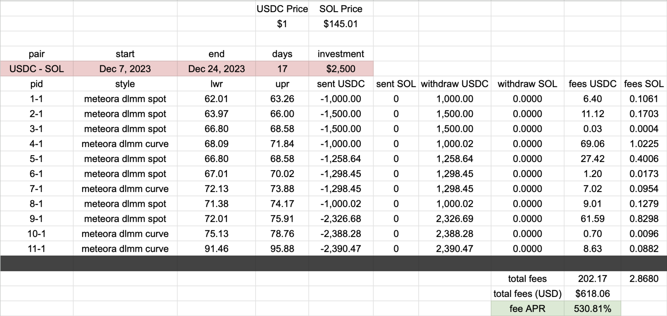 To calculate the overall Fee APR, I first aggregate the fees, viewing the 11
positions as a single one: I put up $2500 and earned 202.17 USDC and 2.868 SOL
over 17 days. I then calculate the USD value of these fees at current prices.
For example, the price of SOL was $145.01 at the time of the writing, making
the fees worth $618.06 in total. Finally, I plug the numbers into method 1 to
get the overall Fee APR: \(\frac{618.06}{2500}*\frac{365}{17} = 530.81\%\).
To calculate the overall Fee APR, I first aggregate the fees, viewing the 11
positions as a single one: I put up $2500 and earned 202.17 USDC and 2.868 SOL
over 17 days. I then calculate the USD value of these fees at current prices.
For example, the price of SOL was $145.01 at the time of the writing, making
the fees worth $618.06 in total. Finally, I plug the numbers into method 1 to
get the overall Fee APR: \(\frac{618.06}{2500}*\frac{365}{17} = 530.81\%\).
6.1 Capital Gains or Losses
LPs earn fees by taking on price risk. Price fluctuations automatically sell one token for the other in a liquidity pool. In the worst-case scenario-if you pair a good coin with a shit coin-you will end up with 100% of the shit coin in your position as its price crashes and your position will be worthless.
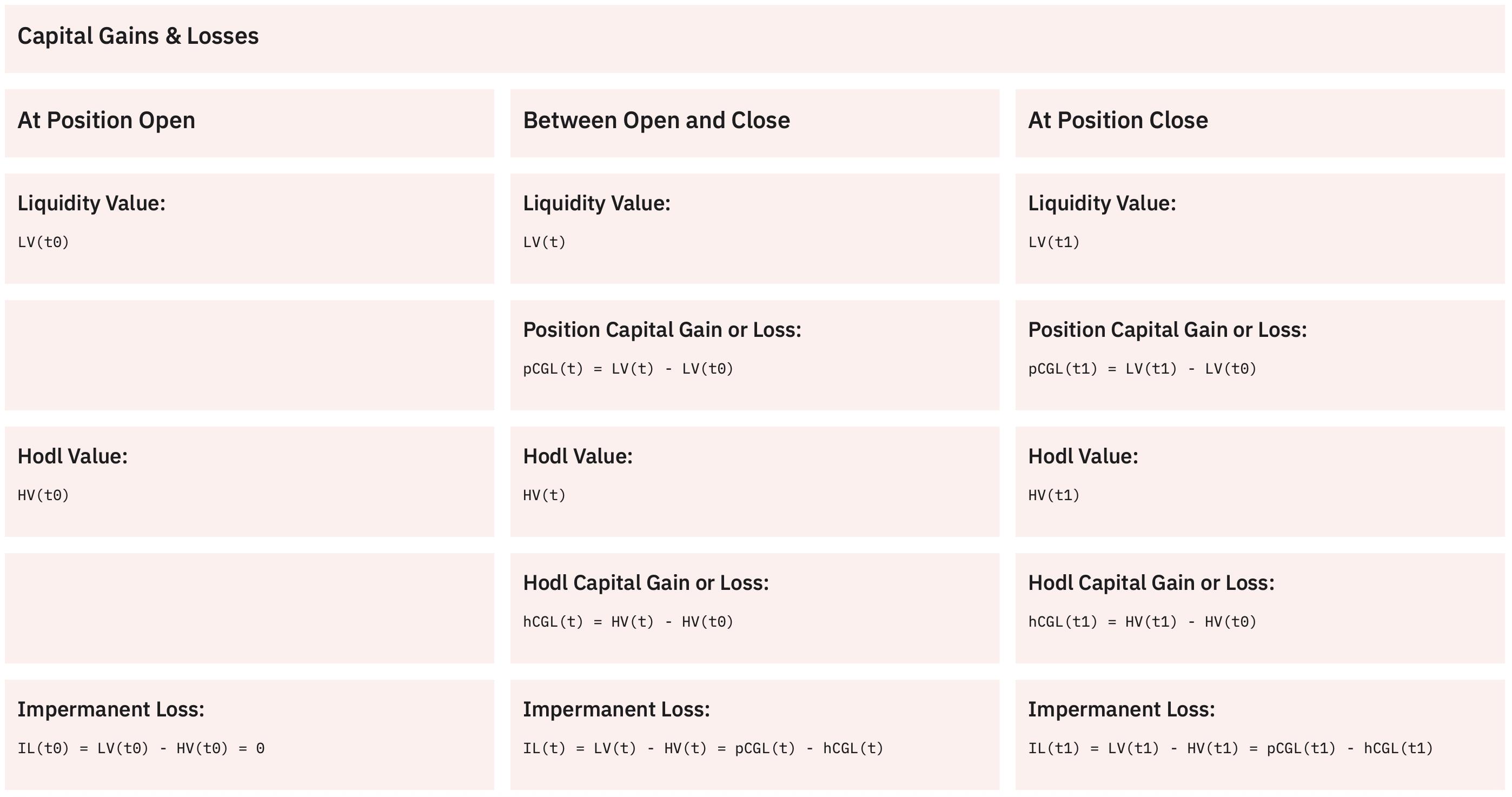
At any point in time, we want to know the USD value of our position and measure how it has changed since the beginning. Specifically, we need these metrics:
- position Capital Gains or Losses (pCGL) = Current Liquidity Value - Initial Liquidity Value.
- hodl Capital Gains or Losses (hCGL) = Current Hodl Value - Initial Hodl Value.
Mathematically, these can be written as
- \(pCGL(t) = LV(t) - LV(t_0)\), where \(LV\) stands for Liquidity Value.
- \(hCGL(t) = HV(t) - HV(t_0)\), where \(HV\) stands for Hodl Value.
If we compare liquidity value and hodl value (at the same time point), we get Impermanent Loss (IL), i.e., Impermanent Loss (IL) = Current Liquidity Value - Current Hodl Value, which can be written mathematically as \(IL(t) = LV(t) - HV(t)\).
On the other hand, IL is equal to the difference between position and hodl Capital Gains or Losses. To see this, just plug in their definitions: \(pCGL(t) - hCGL(t) = (LV(t) - LV(t_0)) - (HV(t) - HV(t_0)) = LV(t) - HV(t) + (HV(t_0) - LV(t_0))\), but \(HV(t_0) - LV(t_0) = 0\) because Initial Hodl Value is the same as Initial Liquidity Value, so \(pCGL(t) - hCGL(t) = LV(t) - HV(t) = IL(t)\).
Let’s organize these capital gains or losses formulas chronologically.
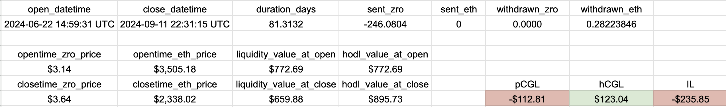
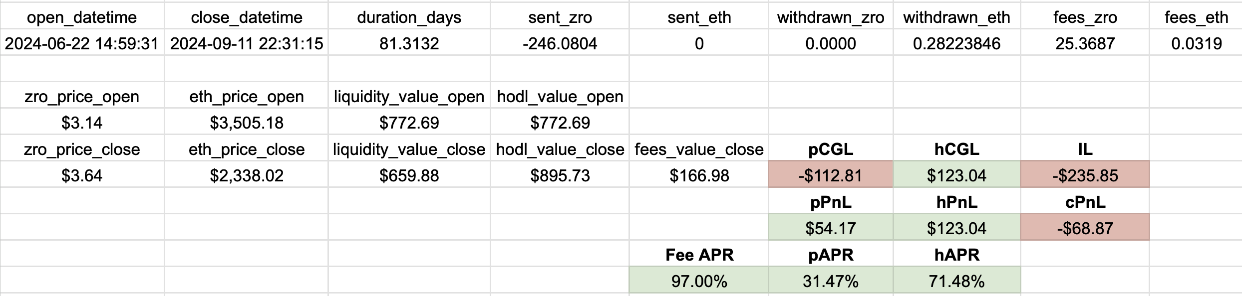
And let’s calculate pCGL, hCGL, and IL at position close time for the same
ZRO-ETH position mentioned above. As shown in the below screen, the position has
a capital loss of $112.81 due to ZRO’s price appreciation against ETH. We would
have made $235.85 more (ignoring swap fees) by holding the ZRO tokens in a
wallet and selling them at $3.64 for USDC.
6.2 PnL & ROI
Continuing with the same example and assuming gas is 0, let’s now add swap fees and calculate the PnL and ROI for the ZRO-ETH LP position and the ZRO-hodling case respectively. The $166.98 in fees earned offset the $112.81 capital loss, resulting in a position PnL (pPnL) of $54.17, which is $68.87 less than the hodl PnL (hPnL). Despite generating fees at an impressive 97% annualized rate over more than 81 days, the LP position failed to outperform simply holding and selling ZRO at its peak. The LP’s ROI came to 31.47% APR, significantly trailing the 71.48% APR from holding.
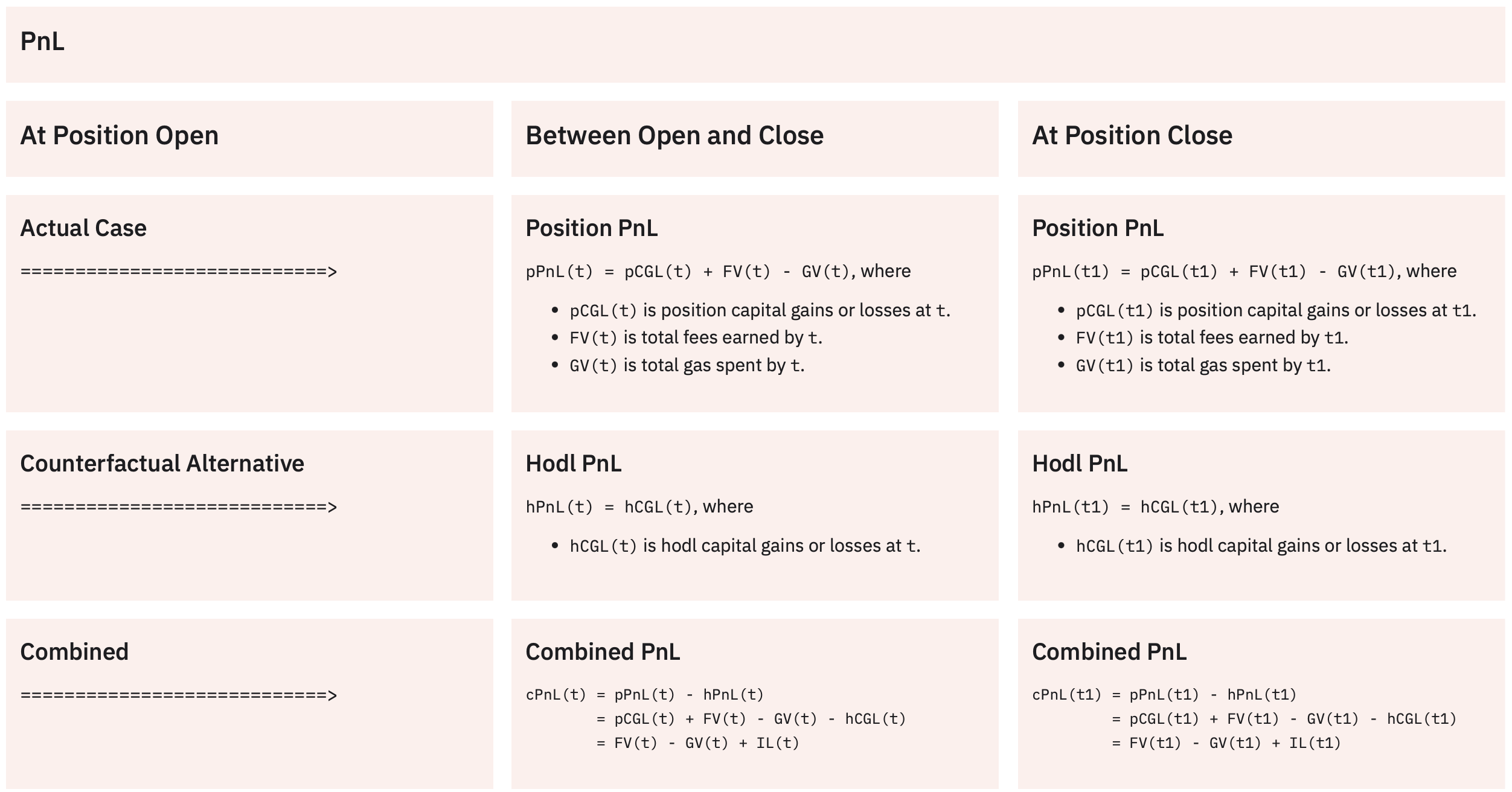
Let’s formalize the metrics mentioned in the previous paragraph:
- position PnL (pPnL) = Current Liquidity Value - Initial Liquidity Value + Fees Earned - Gas.
- hodl PnL (hPnL) = hodl Capital Gains or Losses (hCGL).
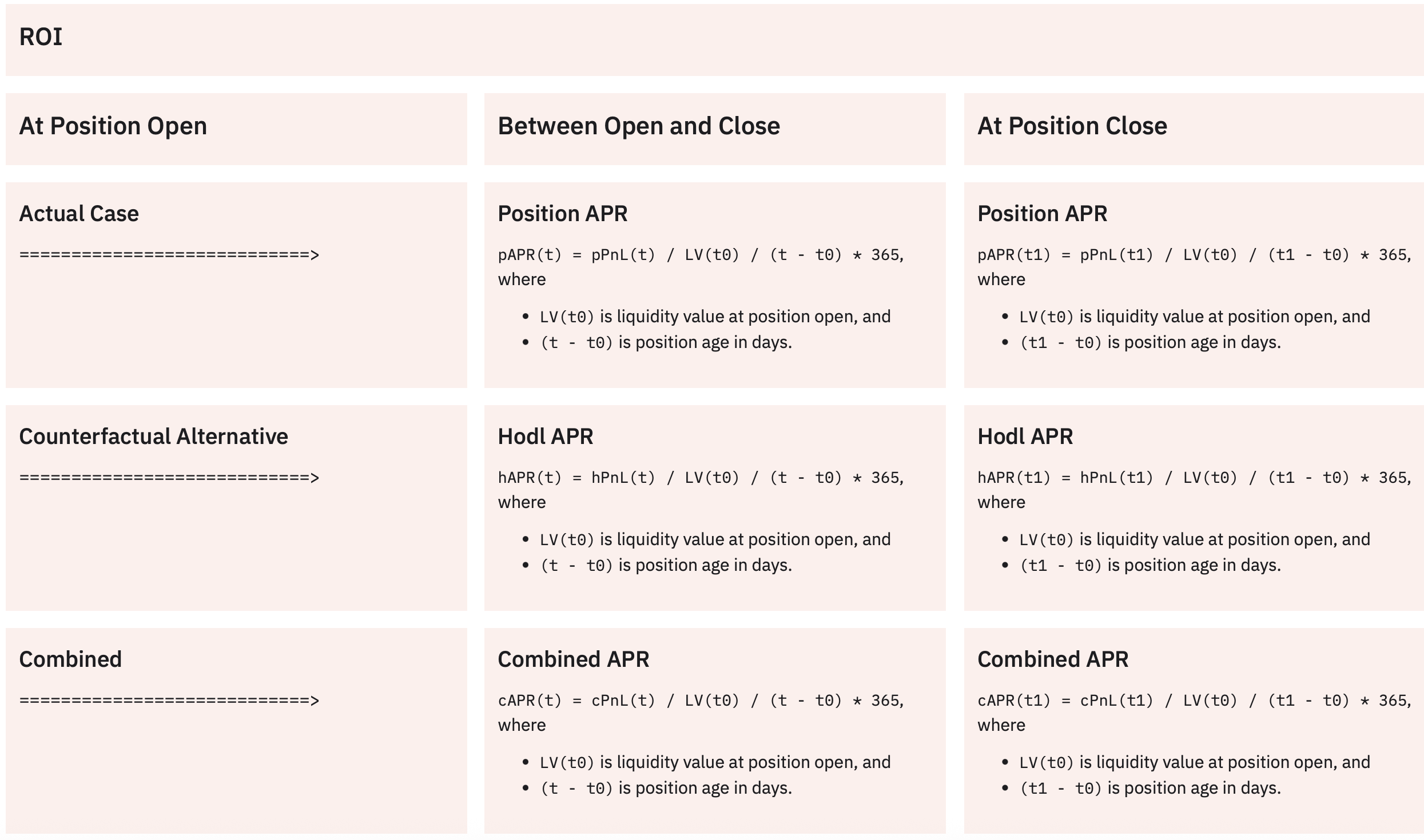
- position APR (pAPR) = Position PnL / Initial Liquidity Value / Position Age (days) * 365.
- hodl APR (hAPR) = hodl PnL / Initial Hodl Value / Position Age (days) * 365.
Mathematically, these can be written as
- \(pPnL(t) = LV(t) - LV(t_0) + Fees(t) - Gas\), where \(LV\) stands for Liquidity Value.
- \(hPnL(t) = hCGL(t)\).
- \(pAPR(t) = \frac{pPnL(t)}{LV(t_0)} * \frac{365}{days}\).
- \(hAPR(t) = \frac{hPnL(t)}{HV(t_0)} * \frac{365}{days}\). Note \(HV(t_0) = LV(t_0)\).
By entering an LP position, we realize the position PnL but forfeit the hodl PnL. To assess the net impact, we can combine the two as follows:
- combined PnL (cPnL) = position PnL - hodl PnL.
- combined APR (cAPR) = combined PnL / Initial Liquidity Value / Position Age (days) * 365.
mathematically written as
- \(cPnL(t) = pPnL(t) - hPnL(t)\).
- \(cAPR(t) = \frac{cPnL(t)}{LV(t_0)} * \frac{365}{days}\).
These formulas are organized chronologically in the two screens below.
I usually ignore the combined PnL and APR metrics because they are distracting at best and harmful at worst21. Unfortunately, revert finance labels them as “total PnL” and “total APR” and displays them prominently.
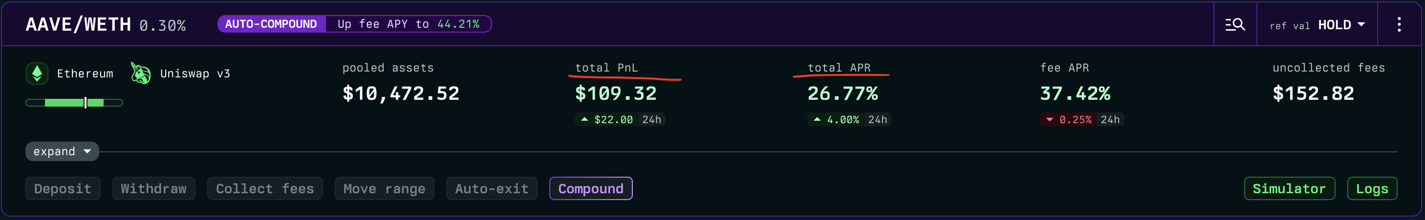
This is misleading since people typically use “total PnL” or “total return” to mean realized net earnings while ignoring the opportunity cost of capital. For example, when calculating the total return of your stocks portfolio, you don’t say, “well, instead of buying stocks, I could’ve held cash, bought a house, went back to school, or aped into Bitcoin. Let me calculate the conterfactual return of each opportunity I didn’t pursue and subtract them in my final return’s calculation.” Plus, the combined PnL and APR only account for one opportunity cost (hodling) and not all possible opportunities. So you should ignore “total PnL” or “total return” reported on revert finance.
A corollary of ignoring combined PnL and APR is to also disregard hodl PnL and APR. I only use position PnL and APR as the definitive performance metrics. So if someone asks me, “How well did you do on your LP positions?” I will add up the pPnLs of these positions and calculate their total pAPR. In the next chapter, I will explain how to do this and share some googlesheets I made. But for now, say my calculation shows I made $500 over 2 months on $5000 (60.8% APR). That person will probably say, “Not bad. What’s your impermanent loss?” To which I’ll respond: “I don’t know - and I don’t care.” Although I’ve already explained myself in section 4.2, in the next chapter, I will continue to explain why impermanent loss doesn’t concern me and why it shouldn’t concern you either. See you in the next chapter.
Welcome
Log in to access this book.