Chapter 3 Deconstructing LP Returns

The total return of any financial asset is composed of two components: capital gains or losses and income. While investors tend to focus on just one component based on their financial literacy and risk appetite, an asset’s true performance can only be measured by looking at the sum of both.

Any asset can exhibit virtually any combination of this mix, depending on how its price behaves relative to the cash flow it generates. At one extreme, some high-growth tech stocks pay zero dividends but experience massive price rallies; some primary residences generate no rental income while their market values steadily depreciate. For decades, Japanese government bonds paid near-zero or negative interest rates while their principal values fluctuated on macro shifts. At the other end of the spectrum, high-yield “dividend traps” promise massive payouts even as their share prices tank, whereas bank CDs and high-yield savings accounts offer steady interest with absolute principal stability.

Ultimately, obsessing over yield while ignoring capital losses–or chasing price action while ignoring cash flow–is a recipe for poor total return. Whether we are buying stocks, bonds, real estate, or providing liquidity in an AMM pool, it is the combined effect of capital gains or losses and income that dictates whether we will walk away with a profit.

For an LP position, its capital gains or losses are driven by the price movements of the underlying token pair, while income accumulates continuously from the swap fees. Evaluating either component in isolation gives a dangerously misleading picture of the position’s total return and actual health.

This chapter is divided into three parts, introducing symbols and equations to formalize each metric and describe their relationships:

Capital Gains or Losses: Maps out price performance for both LP and HODL positions, demonstrating that their difference equals Impermanent Loss (IL).
Fee Income: Focuses on the pool’s earning power, presenting the formula to calculate Fee APR.
Profit and Loss: Brings these two halves together and calculates Profit and Loss (PnL) and the overall Return on Investment (ROI).

3.1 Capital Gains or Losses

Liquidity providers take on significant price risk. Because an AMM pool automatically sells the winner for the loser as prices fluctuate, a worst-case scenario occurs when pairing a fundamentally strong asset with a collapsing one. In that event, the position will eventually end up with 100% of the crashing asset, rendering the total position virtually worthless.

To evaluate performance, an investor must track the USD value of the position and measure how it changes over time relative to the HODL benchmark. This requires two metrics:

Position Capital Gains or Losses ($pCGL$): The change in the value of the underlying assets in a liquidity position.
HODL Capital Gains or Losses ($hCGL$): The change in the value of the underlying assets had they been held in a wallet.

Mathematically, these metrics are defined as:

\[pCGL(t) = LV(t) - LV(t_0)\]
\[hCGL(t) = HV(t) - HV(t_0)\]

Where $LV$ is Liquidity Value, $HV$ is HODL Value, $t_0$ is the initial deployment timestamp, and $t$ is the current time.

Comparing the liquidity position’s value to the counterfactual HODL value at any given time yields Impermanent Loss (IL):

Impermanent Loss = Current Liquidity Value - Current HODL Value
\[IL(t) = LV(t) - HV(t)\]

Alternatively, Impermanent Loss (IL) can be expressed as the difference between the position’s capital gains or losses and the HODL capital gains or losses. Plugging their definitions into the equation demonstrates this relationship:

\[ \begin{aligned} pCGL(t) - hCGL(t) &= (LV(t) - LV(t_0)) - (HV(t) - HV(t_0))\\ &= LV(t) - HV(t) + (HV(t_0) - LV(t_0)) \end{aligned} \]

Because the initial HODL value is identical to the position’s initial liquidity value at the moment of deployment ($HV(t_0) - LV(t_0) = 0$), the equation simplifies perfectly:

\[ pCGL(t) - hCGL(t) = LV(t) - HV(t) = IL(t) \]

As an example, let’s calculate $pCGL$, $hCGL$, and $IL$ for a one-sided ZRO-ETH position that was entered with only ZRO from the bottom of its price range. Important data about the position–including opening and closing timestamps, duration, asset quantities, and token prices–is detailed in the screenshot below. This data is used to determine the initial and final values of the liquidity position and the counterfactual HODL benchmark.

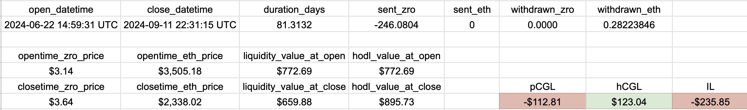
According to the data, this position incurred a capital loss ($pCGL$) of $112.81. The LP would have made $235.85 more (excluding swap fees) by simply holding the initial ZRO tokens and selling them at the moment of closure when the price of ZRO was at $3.64.

3.2 Fee Income

Liquidity providers seek to maximize fee income to offset price risk. For any given liquidity position at time $t$, there are two primary methods for calculating its Fee APR:

Initial-Value Fee APR: Measures fee income relative to the position’s starting value.
Current-Value Fee APR: Measures fee income relative to the current value of the underlying assets in the position.

Mathematically, these metrics are defined as:

\[Fee\text{ }APR(t)=\frac{FV(t)}{LV(t_0)}\times\frac{365}{days}\]
\[Fee\text{ }APR(t)=\frac{FV(t)}{LV(t)}\times\frac{365}{days}\]

Where

$FV(t)$ is the Fees Value, representing the USD value of all fees earned up to
time $t$.
$LV(t_0)$ is the initial Liquidity Value, representing the USD value of capital deployed at the position’s opening timestamp $t_0$.
$LV(t)$ is the current Liquidity Value, representing the USD value of tokens in the position at time $t$.
$\text{days}$ is the duration the position has been active, calculated as $(t - t_0) / 86400$, assuming $t$ and $t_0$ are measured in seconds.

💡 Note on Liquidity Modifications

Formula 1 assumes a static deposit and zero withdrawal. If liquidity is added to or partially withdrawn from a live position, the original baseline ($LV(t_0)$) is altered mid-flight. This makes Formula 1 invalid unless the capital baseline is mathematically time-weighted.

Let’s calculate the Fee APR at position closure ($t_1$). To perform this calculation, we must first track a few items:

Opening and closing timestamps ($t_0$ and $t_1$)
Token prices at both the opening and closing timestamps
The quantity of tokens deposited at opening
The quantity of principal tokens withdrawn at closing
The total amount of fees collected for each token

The values of these items for the ZRO-ETH position mentioned before are collected in the screenshot below:

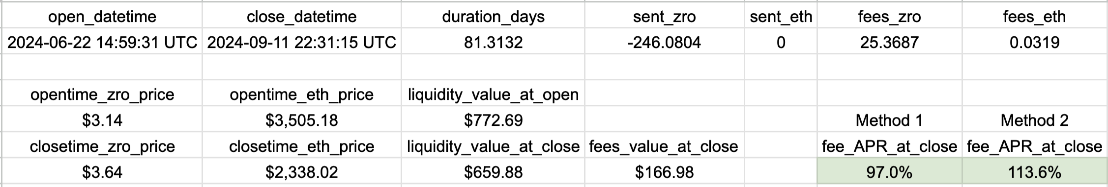
Using these raw inputs, we then compute the following intermediate metrics:

The duration of the position (expressed in days)
The total Fees Value ($FV(t_1)$) evaluated at the closing timestamp $t_1$
The initial Liquidity Value ($LV(t_0)$) and final Liquidity Value ($LV(t_1)$)

Finally, calculating the position’s Fee APR at closure yields 97% under Formula 1 and 113.6% under Formula 2, as displayed in the screenshot.

While Formula 1 is often preferred for performance tracking because it accurately measures yield against the investor’s original capital deployment, Formula 2 is far more convenient to compute programmatically because it removes the requirement to query historical token prices at $t_0$. Consequently, the vast majority of DEXs utilize a variant of Formula 2 for real-time Fee APR displays. Because Fee APR is primarily used to compare different positions or pools, this methodological variance is acceptable–consistency across comparisons matters far more than the absolute percentages themselves.

In practice, it is rarely necessary to calculate the Fee APR of an individual position since most DEXs display it automatically. For Uniswap V3, tracking tools like Revert Finance (https://revert.finance) can monitor individual positions in real time.

However, manual calculation becomes essential when trying to determine the aggregate Fee APR across multiple positions. For instance, the screenshot below details a sequence of 11 USDC-SOL positions that were live between December 7 and 24, 2023. This sequence began with an initial capital of $2,500. The final two columns record the fees earned in both USDC and SOL for each position.

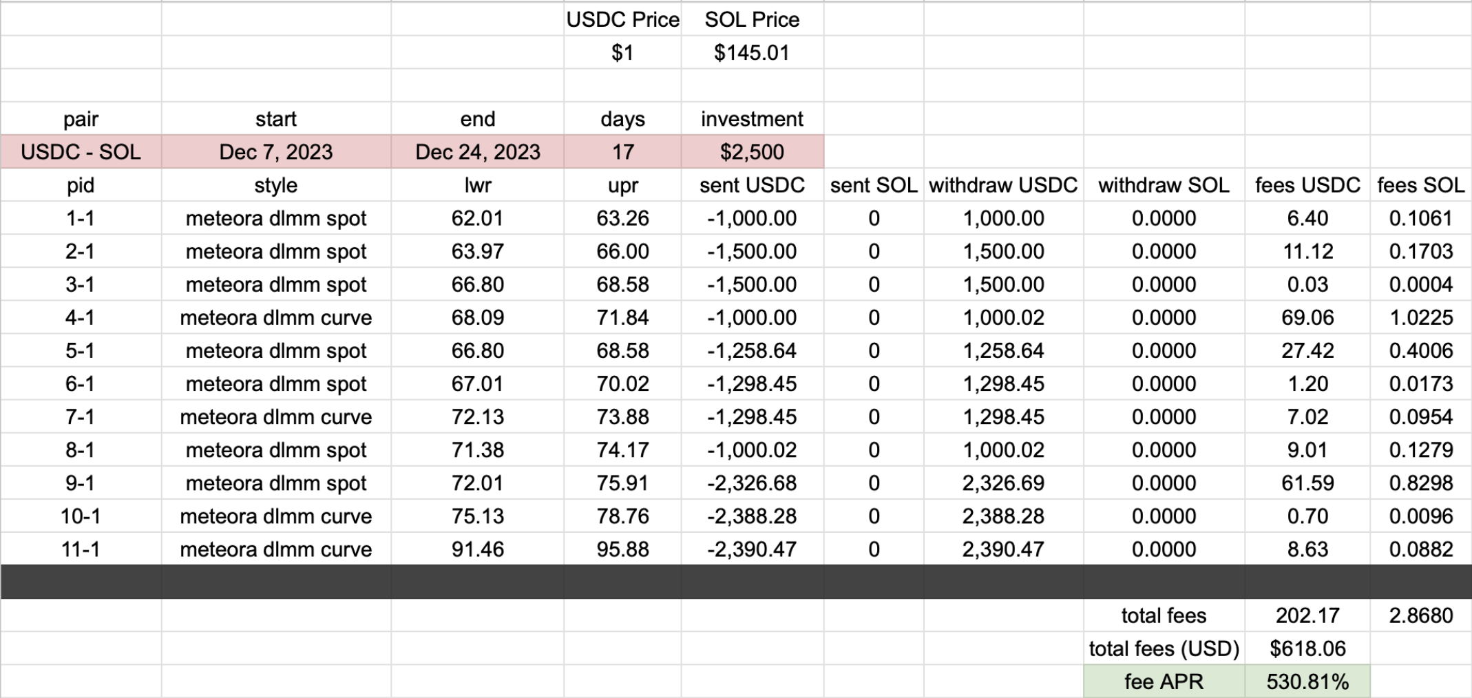
To calculate the overall Fee APR, we first aggregate the fees to yield cumulative earnings of 202.17 USDC and 2.868 SOL over a duration of 17 days. Next, we determine the total Fees Value ($FV(t_1)$) by converting these earnings into USD. For this calculation, assuming a SOL price of $145.01 establishes the total value of the fees at $618.06. Finally, we can plug these values, along with the initial capital outlay of $2500, into Formula 1 to calculate the aggregate Fee APR: \[\frac{618.06}{2500}*\frac{365}{17} = 530.81\%\]

3.3 Profit and Loss (PnL)

Evaluating the performance of an LP position requires looking beyond isolated metrics. A position can generate exceptional fee income while simultaneously losing more value due to adverse price movements in the underlying tokens. Conversely, a position that doesn’t accumulate a lot of fees in the short term might turn a substantial profit simply because the deposited tokens skyrocketed in value. The former scenario leads to net losses, which we want to avoid at all costs, while the latter results in a profit, though it leaves us with a missed opportunity for higher gains–an annoying outcome, but one we can live with–since no one goes bankrupt by taking profits.

To find the ground truth, we must bring token price fluctuations, fee income, and transaction costs together to calculate Position performance (how the LP strategy fared) and compare it against HODL performance (the benchmark of what would have happened if we simply held the tokens in a wallet).

Ultimate Performance Metrics

Position PnL ($pPnL$): The net profit or loss of the LP position, accounting for capital gains or losses on the principal tokens, total fees earned, and gas subtracted as transaction costs²⁸.
HODL PnL ($hPnL$): The net profit or loss of the benchmark, representing the capital gains or losses realized if the initial tokens had simply been held statically in a wallet.
Position APR ($pAPR$): The annualized rate of return of the LP position, relative to the initial deployed capital.
HODL APR ($hAPR$): The annualized rate of return of the HODL benchmark, relative to its initial value.

Mathematically, assuming the LP position’s duration is calculated from Unix timestamps as $\text{days} = (t - t_0) / 86400$, these metrics are defined as:

\[pPnL(t) = pCGL(t) + FV(t) - Gas\]
\[hPnL(t) = hCGL(t)\]
\[pAPR(t) = \frac{pPnL(t)}{LV(t_0)} \times \frac{365}{days}\]
\[hAPR(t) = \frac{hPnL(t)}{HV(t_0)} \times \frac{365}{days}\]

Where $HV(t_0) = LV(t_0)$, representing the identical starting value of both the LP strategy and the HODL benchmark.

In addition, by entering an LP position, we realize the Position PnL but forfeit the HODL PnL on the same capital. To capture this opportunity cost, we can further combine the two metrics:

Combined PnL ($cPnL$): The difference between the LP strategy and the HODL benchmark.

\[cPnL(t) = pPnL(t) - hPnL(t)\]

Combined APR ($cAPR$): The annualized rate of return of choosing LP over HODL.

\[cAPR(t) = pAPR(t) - hAPR(t)\]

The following screenshot displays these ultimate performance metrics for the ZRO-ETH position, assuming gas costs were zero.

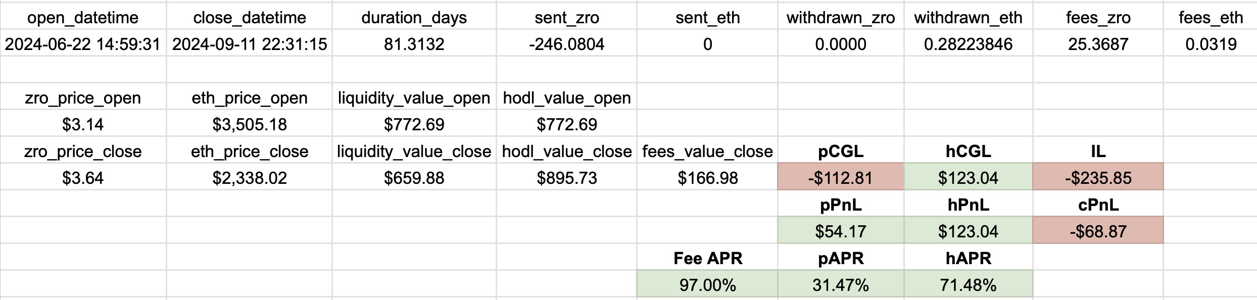In this case, $166.98 in fee income offset -$112.81 in capital losses, resulting in a positive Position PnL ($pPnL$) of $54.17. However, this trailed the HODL PnL ($hPnL$), yielding a negative Combined PnL ($cPnL$) of -$68.87. Despite generating fees at an impressive 97% annualized rate over an 81-day period, the LP position failed to outperform HODL. It yielded a Position APR ($pAPR$) of 31.47%, significantly trailing the 71.48% HODL APR ($hAPR$), resulting in a Combined APR ($cAPR$) of -40.01%.

💡 Terminology Warning: Combined vs. Total

Some DeFi analytics platforms, notably Revert Finance, use the terms “Total PnL” and “Total APR” instead of “Combined PnL” and “Combined APR.” This naming convention is confusing, as investors typically use “total PnL” or “total return” to mean the direct final outcome of an investment strategy without considering any missed opportunities.

3.4 The LP Reality Check

Most people become liquidity providers because they want to put their capital to work. Attracted by the high yields offered by AMMs, they jump in without considering capital losses–and end up getting rekt. An LP position can pull in staggering fees while still netting a negative PnL due to collapsing token prices, making it dangerous to focus solely on fee generation. Even if an LP position is profitable, there’s always the question of whether more could have been earned by simply letting the tokens sit in a wallet. More often than not, a position can turn a solid profit while still quietly underperforming buy-and-hold.

By utilizing the Position, HODL, and Combined metrics defined in this chapter, we can cut through the noise and accurately determine whether an LP position is adding value:

Position Metrics ($pPnL$ / $pAPR$): Measure the return of the deployed capital, disregarding any opportunity costs.
HODL Metrics ($hPnL$ / $hAPR$): Establish a benchmark of a passive buy-and-hold strategy for comparison.
Combined Metrics ($cPnL$ / $cAPR$): Deliver the awakening reality check, revealing whether the LP strategy simply introduced smart-contract risk for a return inferior to buy-and-hold.

But knowing these calculations is not enough for designing a successful LP strategy. To survive and thrive, liquidity providers must ingrain in their blood the primary force that drives these metrics into negative territory. In the next chapter, we will look at exactly how collapsing token prices unravel the highest-yielding pools and break down why so many “lucrative” AMM pools are actually capital-sucking black holes.

Transaction costs should also include any expenses incurred from onramping, offramping, or bridging assets.↩︎

Liquidity Provision Mastery: Strategies for AMMs and Yield Optimization.

Chapter 3 Deconstructing LP Returns

3.1 Capital Gains or Losses

3.2 Fee Income

3.3 Profit and Loss (PnL)

3.4 The LP Reality Check

Welcome